MCMC Sampling

The CmdStanModel class method sample invokes Stan’s adaptive HMC-NUTS sampler which uses the Hamiltonian Monte Carlo (HMC) algorithm and its adaptive variant the no-U-turn sampler (NUTS) to produce a set of draws from the posterior distribution of the model parameters conditioned on the data. It returns a CmdStanMCMC object which provides properties to retrieve information about the sample, as well as methods to run CmdStan’s summary and diagnostics tools.

In order to evaluate the fit of the model to the data, it is necessary to run several Monte Carlo chains and compare the set of draws returned by each. By default, the sample command runs 4 sampler chains, i.e., CmdStanPy invokes CmdStan 4 times. CmdStanPy uses Python’s subprocess and multiprocessing libraries to run these chains in separate processes. This processing can be done in parallel, up to the number of processor cores available.

Prerequisites

CmdStanPy displays progress bars during sampling via use of package tqdm. In order for these to display properly, you must have the ipywidgets package installed, and depending on your version of Jupyter or JupyterLab, you must enable it via command:

!jupyter nbextension enable --py widgetsnbextension

Enabling notebook extension jupyter-js-widgets/extension...
      - Validating: OK

For more information, see the the installation instructions, also this tqdm GitHub issue.

Fitting a model to data

In this example we use the CmdStan example model bernoulli.stan and data file bernoulli.data.json.

We instantiate a CmdStanModel from the Stan program file

import os
from cmdstanpy import CmdStanModel, cmdstan_path

bernoulli_dir = os.path.join(cmdstan_path(), 'examples', 'bernoulli')
stan_file = os.path.join(bernoulli_dir, 'bernoulli.stan')
data_file = os.path.join(bernoulli_dir, 'bernoulli.data.json')

# instantiate, compile bernoulli model
model = CmdStanModel(stan_file=stan_file)

INFO:cmdstanpy:compiling stan file /home/docs/checkouts/readthedocs.org/user_builds/cmdstanpy/conda/v1.0.0rc3/bin/cmdstan/examples/bernoulli/bernoulli.stan to exe file /home/docs/checkouts/readthedocs.org/user_builds/cmdstanpy/conda/v1.0.0rc3/bin/cmdstan/examples/bernoulli/bernoulli
INFO:cmdstanpy:compiled model executable: /home/docs/checkouts/readthedocs.org/user_builds/cmdstanpy/conda/v1.0.0rc3/bin/cmdstan/examples/bernoulli/bernoulli

By default, the model is compiled during instantiation. The compiled executable is created in the same directory as the program file. If the directory already contains an executable file with a newer timestamp, the model is not recompiled.

We run the sampler on the data using all default settings: 4 chains, each of which runs 1000 warmup and sampling iterations.

# run CmdStan's sample method, returns object `CmdStanMCMC`
fit = model.sample(data=data_file)

INFO:cmdstanpy:CmdStan start procesing

INFO:cmdstanpy:CmdStan done processing.

The sample method returns a CmdStanMCMC object, which contains: - metadata - draws - HMC tuning parameters metric, step_size

print('sampler diagnostic variables:\n{}'.format(fit.metadata.method_vars_cols.keys()))
print('stan model variables:\n{}'.format(fit.metadata.stan_vars_cols.keys()))

sampler diagnostic variables:
dict_keys(['lp__', 'accept_stat__', 'stepsize__', 'treedepth__', 'n_leapfrog__', 'divergent__', 'energy__'])
stan model variables:
dict_keys(['theta'])

fit.summary()

	Mean	MCSE	StdDev	5%	50%	95%	N_Eff	N_Eff/s	R_hat
name
lp__	-7.30	0.0210	0.74	-8.800	-7.00	-6.70	1300.0	14000.0	1.0
theta	0.25	0.0031	0.12	0.074	0.23	0.46	1400.0	16000.0	1.0

The sampling data from the fit can be accessed either as a numpy array or a pandas DataFrame:

print(fit.draws().shape)
fit.draws_pd().head()

(1000, 4, 8)

	lp__	accept_stat__	stepsize__	treedepth__	n_leapfrog__	divergent__	energy__	theta
0	-8.18109	0.947147	1.08292	2.0	3.0	0.0	8.18115	0.085541
1	-9.25583	0.960750	1.08292	2.0	3.0	0.0	9.28633	0.054002
2	-8.48709	1.000000	1.08292	1.0	1.0	0.0	9.27267	0.074519
3	-8.60606	0.986149	1.08292	1.0	1.0	0.0	8.88402	0.070754
4	-7.83236	1.000000	1.08292	1.0	1.0	0.0	8.54461	0.101193

Additionally, if xarray is installed, this data can be accessed another way:

fit.draws_xr()

<xarray.Dataset>
Dimensions:  (draw: 1000, chain: 4)
Coordinates:
  * chain    (chain) int64 1 2 3 4
  * draw     (draw) int64 0 1 2 3 4 5 6 7 8 ... 992 993 994 995 996 997 998 999
Data variables:
    theta    (chain, draw) float64 0.08554 0.054 0.07452 ... 0.1688 0.2943
Attributes:
    stan_version:        2.28.1
    model:               bernoulli_model
    num_draws_sampling:  1000

The fit object records the command, the return code, and the paths to the sampler output csv and console files. The string representation of this object displays the CmdStan commands and the location of the output files.

Output filenames are composed of the model name, a timestamp in the form YYYYMMDDhhmm and the chain id, plus the corresponding filetype suffix, either ‘.csv’ for the CmdStan output or ‘.txt’ for the console messages, e.g. bernoulli-201912081451-1.csv. Output files written to the temporary directory contain an additional 8-character random string, e.g. bernoulli-201912081451-1-5nm6as7u.csv.

fit

CmdStanMCMC: model=bernoulli chains=4['method=sample', 'algorithm=hmc', 'adapt', 'engaged=1']
 csv_files:
        /tmp/tmpba1_ahip/bernoulli-20211119014442_1.csv
        /tmp/tmpba1_ahip/bernoulli-20211119014442_2.csv
        /tmp/tmpba1_ahip/bernoulli-20211119014442_3.csv
        /tmp/tmpba1_ahip/bernoulli-20211119014442_4.csv
 output_files:
        /tmp/tmpba1_ahip/bernoulli-20211119014442_0-stdout.txt
        /tmp/tmpba1_ahip/bernoulli-20211119014442_1-stdout.txt
        /tmp/tmpba1_ahip/bernoulli-20211119014442_2-stdout.txt
        /tmp/tmpba1_ahip/bernoulli-20211119014442_3-stdout.txt

The sampler output files are written to a temporary directory which is deleted upon session exit unless the output_dir argument is specified. The save_csvfiles function moves the CmdStan CSV output files to a specified directory without having to re-run the sampler. The console output files are not saved. These files are treated as ephemeral; if the sample is valid, all relevant information is recorded in the CSV files.

Sampler Progress

Your model make take a long time to fit. The sample method provides two arguments:

• visual progress bar: show_progress=True

• stream CmdStan ouput to the console - show_console=True

To illustrate how progress bars work, we will run the bernoulli model. Since the progress bars are only visible while the sampler is running and the bernoulli model takes no time at all to fit, we run this model for 200K iterations, in order to see the progress bars in action.

fit = model.sample(data=data_file, iter_warmup=100000, iter_sampling=100000, show_progress=True)

INFO:cmdstanpy:CmdStan start procesing

INFO:cmdstanpy:CmdStan done processing.

The Stan language print statement can be use to monitor the Stan program state. In order to see this information as the sampler is running, use the show_console=True argument. This will stream all CmdStan messages to the terminal while the sampler is running.

fit = model.sample(data=data_file, chains=2, parallel_chains=1, show_console=True)

INFO:cmdstanpy:Chain [1] start processing
INFO:cmdstanpy:Chain [1] done processing
INFO:cmdstanpy:Chain [2] start processing
INFO:cmdstanpy:Chain [2] done processing

Chain [1] method = sample (Default)
Chain [1] sample
Chain [1] num_samples = 1000 (Default)
Chain [1] num_warmup = 1000 (Default)
Chain [1] save_warmup = 0 (Default)
Chain [1] thin = 1 (Default)
Chain [1] adapt
Chain [1] engaged = 1 (Default)
Chain [1] gamma = 0.050000000000000003 (Default)
Chain [1] delta = 0.80000000000000004 (Default)
Chain [1] kappa = 0.75 (Default)
Chain [1] t0 = 10 (Default)
Chain [1] init_buffer = 75 (Default)
Chain [1] term_buffer = 50 (Default)
Chain [1] window = 25 (Default)
Chain [1] algorithm = hmc (Default)
Chain [1] hmc
Chain [1] engine = nuts (Default)
Chain [1] nuts
Chain [1] max_depth = 10 (Default)
Chain [1] metric = diag_e (Default)
Chain [1] metric_file =  (Default)
Chain [1] stepsize = 1 (Default)
Chain [1] stepsize_jitter = 0 (Default)
Chain [1] num_chains = 1 (Default)
Chain [1] id = 1 (Default)
Chain [1] data
Chain [1] file = /home/docs/checkouts/readthedocs.org/user_builds/cmdstanpy/conda/v1.0.0rc3/bin/cmdstan/examples/bernoulli/bernoulli.data.json
Chain [1] init = 2 (Default)
Chain [1] random
Chain [1] seed = 50018
Chain [1] output
Chain [1] file = /tmp/tmpba1_ahip/bernoulli-20211119014451_1.csv
Chain [1] diagnostic_file =  (Default)
Chain [1] refresh = 100 (Default)
Chain [1] sig_figs = -1 (Default)
Chain [1] profile_file = profile.csv (Default)
Chain [1] num_threads = 1 (Default)
Chain [1]
Chain [1]
Chain [1] Gradient evaluation took 5e-06 seconds
Chain [1] 1000 transitions using 10 leapfrog steps per transition would take 0.05 seconds.
Chain [1] Adjust your expectations accordingly!
Chain [1]
Chain [1]
Chain [1] Iteration:    1 / 2000 [  0%]  (Warmup)
Chain [1] Iteration:  100 / 2000 [  5%]  (Warmup)
Chain [1] Iteration:  200 / 2000 [ 10%]  (Warmup)
Chain [1] Iteration:  300 / 2000 [ 15%]  (Warmup)
Chain [1] Iteration:  400 / 2000 [ 20%]  (Warmup)
Chain [1] Iteration:  500 / 2000 [ 25%]  (Warmup)
Chain [1] Iteration:  600 / 2000 [ 30%]  (Warmup)
Chain [1] Iteration:  700 / 2000 [ 35%]  (Warmup)
Chain [1] Iteration:  800 / 2000 [ 40%]  (Warmup)
Chain [1] Iteration:  900 / 2000 [ 45%]  (Warmup)
Chain [1] Iteration: 1000 / 2000 [ 50%]  (Warmup)
Chain [1] Iteration: 1001 / 2000 [ 50%]  (Sampling)
Chain [1] Iteration: 1100 / 2000 [ 55%]  (Sampling)
Chain [1] Iteration: 1200 / 2000 [ 60%]  (Sampling)
Chain [1] Iteration: 1300 / 2000 [ 65%]  (Sampling)
Chain [1] Iteration: 1400 / 2000 [ 70%]  (Sampling)
Chain [1] Iteration: 1500 / 2000 [ 75%]  (Sampling)
Chain [1] Iteration: 1600 / 2000 [ 80%]  (Sampling)
Chain [1] Iteration: 1700 / 2000 [ 85%]  (Sampling)
Chain [1] Iteration: 1800 / 2000 [ 90%]  (Sampling)
Chain [1] Iteration: 1900 / 2000 [ 95%]  (Sampling)
Chain [1] Iteration: 2000 / 2000 [100%]  (Sampling)
Chain [1]
Chain [1] Elapsed Time: 0.008 seconds (Warm-up)
Chain [1] 0.013 seconds (Sampling)
Chain [1] 0.021 seconds (Total)
Chain [1]
Chain [1]
Chain [2] method = sample (Default)
Chain [2] sample
Chain [2] num_samples = 1000 (Default)
Chain [2] num_warmup = 1000 (Default)
Chain [2] save_warmup = 0 (Default)
Chain [2] thin = 1 (Default)
Chain [2] adapt
Chain [2] engaged = 1 (Default)
Chain [2] gamma = 0.050000000000000003 (Default)
Chain [2] delta = 0.80000000000000004 (Default)
Chain [2] kappa = 0.75 (Default)
Chain [2] t0 = 10 (Default)
Chain [2] init_buffer = 75 (Default)
Chain [2] term_buffer = 50 (Default)
Chain [2] window = 25 (Default)
Chain [2] algorithm = hmc (Default)
Chain [2] hmc
Chain [2] engine = nuts (Default)
Chain [2] nuts
Chain [2] max_depth = 10 (Default)
Chain [2] metric = diag_e (Default)
Chain [2] metric_file =  (Default)
Chain [2] stepsize = 1 (Default)
Chain [2] stepsize_jitter = 0 (Default)
Chain [2] num_chains = 1 (Default)
Chain [2] id = 2
Chain [2] data
Chain [2] file = /home/docs/checkouts/readthedocs.org/user_builds/cmdstanpy/conda/v1.0.0rc3/bin/cmdstan/examples/bernoulli/bernoulli.data.json
Chain [2] init = 2 (Default)
Chain [2] random
Chain [2] seed = 50018
Chain [2] output
Chain [2] file = /tmp/tmpba1_ahip/bernoulli-20211119014451_2.csv
Chain [2] diagnostic_file =  (Default)
Chain [2] refresh = 100 (Default)
Chain [2] sig_figs = -1 (Default)
Chain [2] profile_file = profile.csv (Default)
Chain [2] num_threads = 1 (Default)
Chain [2]
Chain [2]
Chain [2] Gradient evaluation took 4e-06 seconds
Chain [2] 1000 transitions using 10 leapfrog steps per transition would take 0.04 seconds.
Chain [2] Adjust your expectations accordingly!
Chain [2]
Chain [2]
Chain [2] Iteration:    1 / 2000 [  0%]  (Warmup)
Chain [2] Iteration:  100 / 2000 [  5%]  (Warmup)
Chain [2] Iteration:  200 / 2000 [ 10%]  (Warmup)
Chain [2] Iteration:  300 / 2000 [ 15%]  (Warmup)
Chain [2] Iteration:  400 / 2000 [ 20%]  (Warmup)
Chain [2] Iteration:  500 / 2000 [ 25%]  (Warmup)
Chain [2] Iteration:  600 / 2000 [ 30%]  (Warmup)
Chain [2] Iteration:  700 / 2000 [ 35%]  (Warmup)
Chain [2] Iteration:  800 / 2000 [ 40%]  (Warmup)
Chain [2] Iteration:  900 / 2000 [ 45%]  (Warmup)
Chain [2] Iteration: 1000 / 2000 [ 50%]  (Warmup)
Chain [2] Iteration: 1001 / 2000 [ 50%]  (Sampling)
Chain [2] Iteration: 1100 / 2000 [ 55%]  (Sampling)
Chain [2] Iteration: 1200 / 2000 [ 60%]  (Sampling)
Chain [2] Iteration: 1300 / 2000 [ 65%]  (Sampling)
Chain [2] Iteration: 1400 / 2000 [ 70%]  (Sampling)
Chain [2] Iteration: 1500 / 2000 [ 75%]  (Sampling)
Chain [2] Iteration: 1600 / 2000 [ 80%]  (Sampling)
Chain [2] Iteration: 1700 / 2000 [ 85%]  (Sampling)
Chain [2] Iteration: 1800 / 2000 [ 90%]  (Sampling)
Chain [2] Iteration: 1900 / 2000 [ 95%]  (Sampling)
Chain [2] Iteration: 2000 / 2000 [100%]  (Sampling)
Chain [2]
Chain [2] Elapsed Time: 0.007 seconds (Warm-up)
Chain [2] 0.014 seconds (Sampling)
Chain [2]                0.021 seconds (Total)
Chain [2]
Chain [2]

Running a data-generating model

In this example we use the CmdStan example model data_filegen.stan to generate a simulated dataset given fixed data values.

model_datagen = CmdStanModel(stan_file='bernoulli_datagen.stan')
datagen_data = {'N':300, 'theta':0.3}
fit_sim = model_datagen.sample(data=datagen_data, fixed_param=True)
fit_sim.summary()

INFO:cmdstanpy:compiling stan file /home/docs/checkouts/readthedocs.org/user_builds/cmdstanpy/checkouts/v1.0.0rc3/docsrc/examples/bernoulli_datagen.stan to exe file /home/docs/checkouts/readthedocs.org/user_builds/cmdstanpy/checkouts/v1.0.0rc3/docsrc/examples/bernoulli_datagen
INFO:cmdstanpy:compiled model executable: /home/docs/checkouts/readthedocs.org/user_builds/cmdstanpy/checkouts/v1.0.0rc3/docsrc/examples/bernoulli_datagen
INFO:cmdstanpy:CmdStan start procesing

INFO:cmdstanpy:CmdStan done processing.

	Mean	MCSE	StdDev	5%	50%	95%	N_Eff	N_Eff/s	R_hat
name
lp__	0	NaN	0.0	0	0	0.0	NaN	NaN	NaN
theta_rep	90	0.26	8.1	76	90	100.0	970.0	140000.0	1.0

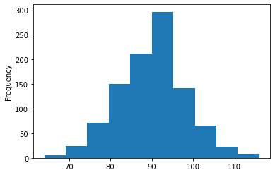
Compute, plot histogram of total successes for N Bernoulli trials with chance of success theta:

drawset_pd = fit_sim.draws_pd()
drawset_pd.columns

# restrict to columns over new outcomes of N Bernoulli trials
y_sims = drawset_pd.drop(columns=['lp__', 'accept_stat__'])

# plot total number of successes per draw
y_sums = y_sims.sum(axis=1)
y_sums.astype('int32').plot.hist(range(0,datagen_data['N']+1))

<AxesSubplot:ylabel='Frequency'>

previous

CmdStanPy Examples

next

Maximum Likelihood Estimation