MCMC Sampling

The CmdStanModel class method sample invokes Stan’s adaptive HMC-NUTS sampler which uses the Hamiltonian Monte Carlo (HMC) algorithm and its adaptive variant the no-U-turn sampler (NUTS) to produce a set of draws from the posterior distribution of the model parameters conditioned on the data. It returns a CmdStanMCMC object which provides properties to retrieve information about the sample, as well as methods to run CmdStan’s summary and diagnostics tools.

In order to evaluate the fit of the model to the data, it is necessary to run several Monte Carlo chains and compare the set of draws returned by each. By default, the sample command runs 4 sampler chains, i.e., CmdStanPy invokes CmdStan 4 times. CmdStanPy uses Python’s subprocess and multiprocessing libraries to run these chains in separate processes. This processing can be done in parallel, up to the number of processor cores available.

Fitting a model to data

In this example we use the CmdStan example model bernoulli.stan and data file bernoulli.data.json.

We instantiate a CmdStanModel from the Stan program file

import os
from cmdstanpy.model import CmdStanModel
from cmdstanpy.utils import cmdstan_path

bernoulli_dir = os.path.join(cmdstan_path(), 'examples', 'bernoulli')
bernoulli_path = os.path.join(bernoulli_dir, 'bernoulli.stan')
bernoulli_data = os.path.join(bernoulli_dir, 'bernoulli.data.json')

# instantiate, compile bernoulli model
bernoulli_model = CmdStanModel(stan_file=bernoulli_path)

INFO:cmdstanpy:compiling stan program, exe file: /home/docs/checkouts/readthedocs.org/user_builds/cmdstanpy/conda/v0.9.77/bin/cmdstan/examples/bernoulli/bernoulli
INFO:cmdstanpy:compiler options: stanc_options={}, cpp_options={}
INFO:cmdstanpy:compiled model file: /home/docs/checkouts/readthedocs.org/user_builds/cmdstanpy/conda/v0.9.77/bin/cmdstan/examples/bernoulli/bernoulli

By default, the model is compiled during instantiation. The compiled executable is created in the same directory as the program file. If the directory already contains an executable file with a newer timestamp, the model is not recompiled.

We run the sampler on the data using all default settings: 4 chains, each of which runs 1000 warmup and sampling iterations.

# run CmdStan's sample method, returns object `CmdStanMCMC`
bern_fit = bernoulli_model.sample(data=bernoulli_data)

INFO:cmdstanpy:start chain 1
INFO:cmdstanpy:start chain 2
INFO:cmdstanpy:finish chain 1
INFO:cmdstanpy:finish chain 2
INFO:cmdstanpy:start chain 3
INFO:cmdstanpy:start chain 4
INFO:cmdstanpy:finish chain 4
INFO:cmdstanpy:finish chain 3

The sample method returns a CmdStanMCMC object, which contains: - metadata - draws - HMC tuning parameters metric, step_size

print('sampler diagnostic variables:\n{}'.format(bern_fit.metadata.method_vars_cols.keys()))
print('stan model variables:\n{}'.format(bern_fit.metadata.stan_vars_cols.keys()))

sampler diagnostic variables:
dict_keys(['lp__', 'accept_stat__', 'stepsize__', 'treedepth__', 'n_leapfrog__', 'divergent__', 'energy__'])
stan model variables:
dict_keys(['theta'])

bern_fit.summary()

	Mean	MCSE	StdDev	5%	50%	95%	N_Eff	N_Eff/s	R_hat
name
lp__	-7.30	0.0170	0.69	-8.700	-7.00	-6.80	1600.0	19000.0	1.0
theta	0.25	0.0033	0.12	0.083	0.24	0.47	1300.0	15000.0	1.0

The sampling data from the fit can be accessed either as a numpy array or a pandas DataFrame:

print(bern_fit.draws().shape)
bern_fit.draws_pd().head()

(1000, 4, 8)

	lp__	accept_stat__	stepsize__	treedepth__	n_leapfrog__	divergent__	energy__	theta
0	-6.77554	0.858660	0.899697	1.0	3.0	0.0	7.30590	0.221467
1	-6.84920	0.992393	0.899697	2.0	3.0	0.0	6.85564	0.308825
2	-7.72500	0.724500	0.899697	1.0	3.0	0.0	8.39493	0.106905
3	-8.91212	0.854331	0.899697	1.0	1.0	0.0	8.91247	0.062149
4	-8.54827	1.000000	0.899697	2.0	3.0	0.0	9.05736	0.072551

Additionally, if xarray is installed, this data can be accessed another way:

bern_fit.draws_xr()

<xarray.Dataset>
Dimensions:  (draw: 1000, chain: 4)
Coordinates:
  * chain    (chain) int64 1 2 3 4
  * draw     (draw) int64 0 1 2 3 4 5 6 7 8 ... 992 993 994 995 996 997 998 999
Data variables:
    theta    (chain, draw) float64 0.2215 0.3088 0.1069 ... 0.1179 0.1663 0.1792
Attributes:
    stan_version:              2.27.0
    model:                     bernoulli_model
    num_unconstrained_params:  1
    num_draws_sampling:        1000

The bern_fit object records the command, the return code, and the paths to the sampler output csv and console files. The string representation of this object displays the CmdStan commands and the location of the output files.

Output filenames are composed of the model name, a timestamp in the form YYYYMMDDhhmm and the chain id, plus the corresponding filetype suffix, either ‘.csv’ for the CmdStan output or ‘.txt’ for the console messages, e.g. bernoulli-201912081451-1.csv. Output files written to the temporary directory contain an additional 8-character random string, e.g. bernoulli-201912081451-1-5nm6as7u.csv.

bern_fit

CmdStanMCMC: model=bernoulli chains=4['method=sample', 'algorithm=hmc', 'adapt', 'engaged=1']
 csv_files:
        /tmp/tmp3vvdloym/bernoulli-202108180205-1-_j9cmhbv.csv
        /tmp/tmp3vvdloym/bernoulli-202108180205-2-3mqnmdqc.csv
        /tmp/tmp3vvdloym/bernoulli-202108180205-3-3_a6buue.csv
        /tmp/tmp3vvdloym/bernoulli-202108180205-4-8g_jnfko.csv
 output_files:
        /tmp/tmp3vvdloym/bernoulli-202108180205-1-_j9cmhbv-stdout.txt
        /tmp/tmp3vvdloym/bernoulli-202108180205-2-3mqnmdqc-stdout.txt
        /tmp/tmp3vvdloym/bernoulli-202108180205-3-3_a6buue-stdout.txt
        /tmp/tmp3vvdloym/bernoulli-202108180205-4-8g_jnfko-stdout.txt

The sampler output files are written to a temporary directory which is deleted upon session exit unless the output_dir argument is specified. The save_csvfiles function moves the CmdStan CSV output files to a specified directory without having to re-run the sampler. The console output files are not saved. These files are treated as ephemeral; if the sample is valid, all relevant information is recorded in the CSV files.

Running a data-generating model using fixed_param=True

In this example we use the CmdStan example model bernoulli_datagen.stan to generate a simulated dataset given fixed data values.

datagen_model = CmdStanModel(stan_file='bernoulli_datagen.stan')
datagen_data = {'N':300, 'theta':0.3}
sim_data = datagen_model.sample(data=datagen_data, fixed_param=True)
sim_data.summary()

INFO:cmdstanpy:compiling stan program, exe file: /home/docs/checkouts/readthedocs.org/user_builds/cmdstanpy/checkouts/v0.9.77/docsrc/examples/bernoulli_datagen
INFO:cmdstanpy:compiler options: stanc_options={}, cpp_options={}
INFO:cmdstanpy:compiled model file: /home/docs/checkouts/readthedocs.org/user_builds/cmdstanpy/checkouts/v0.9.77/docsrc/examples/bernoulli_datagen
INFO:cmdstanpy:start chain 1
INFO:cmdstanpy:finish chain 1

	Mean	MCSE	StdDev	5%	50%	95%	N_Eff	N_Eff/s	R_hat
name
lp__	0	NaN	0.0	0	0	0.0	NaN	NaN	NaN
theta_rep	90	0.25	7.6	77	90	100.0	970.0	140000.0	1.0

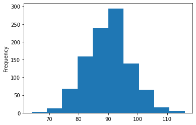
Compute, plot histogram of total successes for N Bernoulli trials with chance of success theta:

drawset_pd = sim_data.draws_pd()
drawset_pd.columns

# restrict to columns over new outcomes of N Bernoulli trials
y_sims = drawset_pd.drop(columns=['lp__', 'accept_stat__'])

# plot total number of successes per draw
y_sums = y_sims.sum(axis=1)
y_sums.astype('int32').plot.hist(range(0,datagen_data['N']+1))

WARNING:matplotlib.font_manager:Matplotlib is building the font cache; this may take a moment.
INFO:matplotlib.font_manager:generated new fontManager

<AxesSubplot:ylabel='Frequency'>

CmdStanPy Examples Maximum Likelihood Estimation